YTEP-0032: Removing the global octree mesh for particle data
Abstract
The global particle octree index used by yt presents a barrier for improving the performance and scalability of visualizing and analyzing particle datasets. This YTEP proposes removing the global octree index, replacing it with a combination of a new IO system and changes to the high-level yt API to focus on returning particle-centric data. The particle I/O refactor makes use of an indexing scheme based on compressed Morton bitmaps which dramatically improves memory usage and scaling for large particle datasets by eliminating the need for a global octree index.
Rather than constructing a global index to maintain backward compatibility at the cost of scaling and performance, we instead propose a reworking of the yt user interface for particle and SPH data to be more “particle-centric”. This means that data object selections for fields that are now defined on the global octree mesh will instead return field data at particle locations. For SPH data, visualizations of slices and projections are done in the image plane, making use of the “scatter” approach by smoothing SPH data directly onto images, employing either a volumetric or projected SPH smoothing kernel. Fully local derived fields are calculated using yt’s existing field definitions but passing in data defined at particle locations. Fields that need spatial derivatives are implemented using the SPH formalism and are also evaluated at the particle locations.
Altogether these changes allow for improved performance and scaling, and allow users to access, analyze, and visualize particle field data for SPH simulations in a more straightforward fashion. While we do not propose substantial API changes for mesh or octree codes, these changes to yt’s field system for particle data imply substantial changes to the meaning of yt’s data selection system for particle data. We discuss the implications of these backward incompatible changes and how we intend to document and manage them in a way that is minimally disruptive to users.
Status
In Progress. The implementation is mostly finished, although there are a few features that still need to be implemented.
Project Management Links
The code can be found in pull request 2382:
https://bitbucket.org/yt_analysis/yt/pull-requests/2382
The C++ compressed bitmap implementation we intend to vendor into yt:
Detailed Description
Background
Currently most user-facing operations on SPH data are produced by interpolating
SPH data onto a volume-filling octree mesh. When support for SPH data was added
to yt in the run-up to the yt-3.0 release, this approach allowed yt to support
SPH data in a way that could reuse the existing infrastructure in yt for octree
data and preserve core assumptions in yt that gas fields must correspond to
a volume-filling AMR structure. While this did make initial support for SPH data
much easier, it also had some downsides. In particular, because the octree was a
single, global object, the memory and CPU overhead of smoothing SPH data onto
the octree can be prohibitive on particle datasets produced by large
simulations. Constructing the octree during the initial indexing phase also
required each particle (albeit, in a 64-bit integer) to be present in memory
simultaneously for a sorting operation, which was memory
prohibitive. Visualizations of slices and projections produced by yt using the
default n_ref and over_refine_factor are somewhat blocky since by
default we use a relatively coarse octree to preserve memory. In addition, since
we construct the global octree based on the positions of all particles,
visualizations that include only one particle type sometimes include “holes” in
regions under-sampled by that particle type.
These cosmetic and semantic issues are jarring to users of SPH codes, who tend to think of data defined at the particle locations rather than sampled onto an adaptive mesh. Making our high-level API focus more on particle-centric data will help to ease the cognitive dissonance felt by users of SPH codes when they work with yt.
Over the past two years, Meagan Lang and Matt Turk implemented a new approach for handling I/O of particle data, based on storing compressed bitmaps containing Morton indices instead of an in-memory octree. This new capability means that the global octree index is now no longer necessary to enable I/O chunking and spatial indexing of particle data in yt.
In this document we describe the approach we take for replacing the global octree index with Morton bitmasks. First, we describe the implementation of the Morton bitmask index, changes to the low-level selector API needed to support the Morton bitmask work, and the testing strategy used for the Morton bitmap indexing scheme. Next we discuss high-level changes to how yt handles particle data, changes to the field system for SPH data, the implementation of the SPH pixelizer system for visualizations, a discussion of deposit fields, and a description of the strategy used to test the new approach for SPH data. We close with a discussion of questions that still need to be tackled before this work can be merged.
Low-Level Implementation
Morton Bitmap Index
The generated index serves to map how the domain is populated by particles in datasets split across multiple files. This way, spatial queries can skip files that do not contain particles in the selected part of the domain. The files are mapped by storing two nested Morton indices for each particle in a dataset. Rather than storing the indices in plaintext, we make use of an EWAH compressed boolean array bitmap. Given a domain with known boundaries in each dimension, a 3-dimension position can be described by a single integer Morton index by
- Dividing the domain into
2^index_order1cells in each dimension with widthsddx = domain_width_x/(2^index_order1). - Determining the 3 integers specifying the cell that contains the 3D
position (e.g.
x/ddx). - Combine the 3 integers into a single integer by alternating bits from each dimension.
These indices can be stored as either integers or in boolean masks. In the case
of the mask, an array of zeroed bits is created with a length equal to the
maximum possible index for the chosen value of index_order1. Then the bits
for the indices present are set to one. To save space, boolean masks in the form
of bitmaps can then be compressed further using the Enhanced Word-Aligned
Hybrid (EWAH) bitmap compression algorithm. In practice, we make use of a
vendored version of EWAHBoolArray,
a C++ EWAH bitmask implementation available under the Apache v2 license.
One bitmap is created for each file. If an index is present in more than one file’s bitmap, this represents a collision and decreases the likelihood that the bitmap can be used to exclude files during spatial queries. This is unlikely if the particles are well partitioned between the files according to a domain decomposition scheme at the chosen order, but this is not generally true of particle datasets produced by astrophysical simulations. In these cases, it is better to create a more refined index.
Using a larger index_order1 increases the refinement of the index, but also
increases both the memory required to store the indices and the time required
to query them for EWAH bitmaps. To combat this, we include a second refined
index within those cells that have indices in multiple files’ bitmaps for the
coarse index. For each particle with a coarse index that collides with another
file, a second refined Morton index is creating by following the same procedure
as for the coarse index, but exchanging the domain boundaries for the boundaries
of the coarse index cell. The refined index for each file is then stored in a
EWAH bitmap for each coarse cell with a collision.
The coarse and refined indices are generated in two separate I/O passes over the
entire dataset. To generate the coarse index, the coordinates of all particles,
as well as the softening lengths for SPH particles, are read in from each
file. For each particle we then compute the Morton index corresponding to the
particles position within the domain. This index, mi is then used to set the
mith element in a boolean mask for the file to 1. If the particle is an
SPH particle, neighboring indices with cells that overlap a sphere with a radius
equal to the particle’s softening length and centered on the particle are also
set to 1.
Once a coarse boolean mask is obtained for each file, the masks are stored in a
set of EWAH compressed bitmaps (implemented in the ewah_bool_array Cython
extension classes). Using logical boolean operations, we then identify those
indices that are set to 1 in more than one file’s mask (the collisions). The
EWAH format is particularly good at logical operations, as it does not
necessarily require decompression to determine whether or not particular bits
are set.
During a second I/O pass over the entire dataset, refined indices are created for those particles with colliding coarse indices. Both the coarse and refined indices are stored in an array for each file. One a file has been completely read in, those indices are sorted and used to create a map from coarse indices to EWAH compressed bitmaps. This is done because entries in EWAH compressed bitmaps must be set in order.
The Morton bitmap index is created for each particle dataset upon its first
ingestion into yt and saved to a sidecar file. At all future ingestions of the
dataset into yt, the index will be loaded from the sidecar file. Indexes are
managed through the Cython extension class ParticleBitmap (defined in
yt/geometry/particle_oct_container.pyx), which is exposed to the user
visible yt API via the regions attribute of the ParticleIndex class
(e.g. ds.index.regions). The ParticleBitmap class generates EWAH bitmaps
via the BoolArrayCollection Cython extension object (defined in
yt/utilities/lib/ewah_bool_wrap.pyx), which wraps the underlying
EWAHBoolArray C++ library.
In the current implementation users can control the creation of the bitmask
index via the index_order and index_filename keyword arguments accepted
by SPHDataset instances. These keyword arguments replace the deprecated
n_ref, over_refine_factor and index_ptype keyword arguments. The
index_order is a two-element tuple corresponding to the maximum Morton order
for the coarse and refined index. Using a tuple for the index_order instead
of two keyword arguments is not only more terse, but it will allow us to produce
bitmask indexes in the future with multiple refined indices while maintaining
the same public API. Currently the default index_order is (7, 5). If a
user specifies index_order as an integer, the integer is taken as the order
of the coarse index and the order of the refined index is set to 1,
producing a trivial refined index. For example:
import yt
ds = yt.load('snapshot_033/snap_033.0.hdf5',
             index_order=(5, 3), index_filename='my_index')
ds.index
Running this script will produce the following output:
yt : [INFO     ] 2017-02-14 11:50:20,815 Allocating for 4.194e+06 particles
Initializing coarse index at order 5: 100%|██████| 12/12 [00:00<00:00, 14.60it/s]
Initializing refined index at order 3: 100%|█████| 12/12 [00:01<00:00,  8.80it/s]
And produce a file named my_index in the same folder as
snapshot_033/snap_033.0.hdf5. The second and all later times the script is
run we only need to load the index from disk, so it produces the following
output:
yt : [INFO     ] 2017-02-14 11:56:07,977 Allocating for 4.194e+06 particles
Loading particle index: 100%|███████████████████| 12/12 [00:00<00:00, 636.33it/s]
Note that there 12 iterations for each loop. Each of these iterations correspond to a single IO chunk. If a file has fewer than 262144 particles, the entire file is used as an IO chunk. If a file has more than 262144 particles, the file is logically split into several subfiles, each containing up to 262144 particles. Currently the chunk size of 262144 particles is hard-coded for all SPH frontends.
Changes to the Selector API
The Morton bitmaps needed for individual data objects are constructed using the
existing low-level Cython selection API. To determine whether a given Morton
index is “contained” in the geometric primitive defined by the selector we make
use of the select_bbox selection API call, since each index corresponds to a
single cell in an octree. If the selector fully encloses the bounding box for
the cell defined by a given Morton index, the existing select_bbox function
is sufficient. However, given that the goal of the Morton bitmap index is to
reduce the number of files we need to read from for a given selection operation,
more care must be taken near the “edges” of a selector. For this reason, we have
added a new function to the selector API, select_bbox_edge. This function is
identical to select_bbox in the case when a bounding box is fully contained
inside of the geometric primitive associated with a selector, simply returning 1
in these cases. However, if the bounding box is only partially contained in the
geometric primitive, select_bbox_edge returns 2, indicating partial
overlap. This is used in the bitmap index code to indicate that the coarse
Morton index does not have sufficient resolution in this region, triggering the
generation of refined Morton indices in this region. These smaller bounding
boxes will have a higher probability of being either fully contained or fully
excluded from a data object, decreasing the probability of a file collision. The
select_bbox_edge function has been implemented for all selectors and if this
YTEP is accepted will be a required part of the API for new selectors in the
future.
In addition to the above change, a more minor change was necessary to the
portion of the selector API used to count and select particles contained in a
given selector. Currently, all particles are assumed to be pointlike, which will
lead to incorrect selections for particles that actually have finite volumes
like SPH particles. To account for this, the signature of the count_points
and select_points functions were changed so that instead of accepting only
single scalar radius for all particles, they can accept an array of possibly
variable radii as well. If non-zero radii are passed in, particle selection
operates via the select_sphere method instead of the select_point method
that is currently used. Since some selectors did not yet have implementations of
select_sphere, we have added new implementations where necessary.
Testing
Testing is provided for both the low level routines controlling access to the bitmap, as well for higher level routines that control bitmap generation. Low level tests are located in yt.utilities.lib.tests.test_geometry_utils. This includes tests of the routines for generating Morton indices from cartesian coordinates, extracting single bit coordinates, and locating neighboring morton indices at the coarse or refined index level both with and without periodic boundary conditions.
Higher level tests are located in yt.geometry.tests.test_particle_octree and include the framework to create test datasets with arbitrary domain decomposition schemes across a specified number of files. Tests are included for creating bitmap indices for datasets with no collisions and all collisions that check the number of coarse and refined cells against known answers. In addition we also provided tests for saving/loading bitmaps and identifying input files for rectangular selections on known domain decomposition schemes.
Removing the Global Octree Mesh
Currently, all I/O operations are mediated via the global octree index. Particles are read in from the output file as needed based on their position in the octree. With the arrival of the compressed bitmap index scheme described above, we no longer need to use the global octree to manage I/O chunking. Making the global octree redundant in this way raises the question about whether the octree is really needed at all.
Currently yt makes a distinction between particle fields and mesh fields. All
SPH-smoothed fields (e.g. ('gas', 'density')) are smoothed onto the global
octree mesh. To make a concrete example, let’s try loading an SPH zoom-in
simulation of a galaxy and ask for the ('gas', 'density') field:
import yt
ds = yt.load('GadgetDiskGalaxy/snapshot_200.hdf5')

ad = ds.all_data()
density = ad['gas', 'density']

print(density.shape)
print(ds.particle_type_counts)
Running this script on the latest development version of yt at time of writing
(abf5a8eff1b2) produces the following output:
(5661944,)
{'PartType0': 4334546,
 'PartType1': 4786616,
 'PartType2': 2333848,
 'PartType3': 0,
 'PartType4': 450921,
 'PartType5': 1149}
On my laptop, this script also takes about 116 seconds to run, with 105 s spent
performing the SPH smoothing operation onto the global octree. Note also how the
number of leaf octs in the octree (5661944) does not match the number of SPH
particles (PartType0). This discrepancy is a common source of initial
confusion for users of SPH codes when they first try to use yt to analyze their
data.
We can ask ourselves whether it makes sense to always smooth data onto the global octree. It makes intuitive sense for users of AMR codes for yt to return data defined on a volume-filling mesh, since the volume filling mesh is the “real” data. However, for SPH data, the global octree mesh is not representative of the “native” data. By making the return value of most yt operations for SPH fields be defined on the octree mesh, yt is not being “true” to the data and also makes it harder than it needs to be to access the particle data as such.
In this YTEP, we propose changing the data object API for SPH data by ensuring that all SPH smoothed fields return data defined at the locations of SPH particles. This means that rather than relying on smoothing data onto the global octree, we will instead always return data defined at the particle locations. This means that running the script included above would produce the following output:
(4334546,)
{'PartType0': 4334546,
 'PartType1': 4786616,
 'PartType2': 2333848,
 'PartType3': 0,
 'PartType4': 450921,
 'PartType5': 1149}
And that the ('gas', 'density') field would merely be an alias to the
('PartType0', 'Density') field available on-disk. Since we no longer need to
smooth data onto the in-memory global octree, this substantially reduces the
memory needed to work with SPH data while simultaneously substantially improving
performance. Just as an example, in the version of the yt that implements this
YTEP, the script at the top of this section requires only 3.3 seconds to run.
The details of how this backward incompatible change to the yt user experience for SPH data will be implemented is detailed below. This includes all design decisions that have been made in the prototype version of yt that implements this YTEP. In addition, there are still several design decisions about how to implement this YTEP that have not yet been decided on. For more details about these issues, see the “Open Questions” section at the bottom of this document.
Identifying the SPH Particle
All of the proposals in this YTEP require that there be special handling for
fields that correspond to the SPH particle type. Currently yt does not have a
way of identifying whether a given particle type in a particle dataset is an SPH
particle. To ameliorate this, we propose adding a new private attribute of
SPHDataset instances, _sph_ptype. This attribute should resolve to the
string name of the SPH particle type for the given output type. For example, for
Gadget HDF5 data, the _sph_ptype is 'PartType0'. Having this attribute
available makes it much easier to write code that does special handling for SPH
data.
SPH Fields
Here we discuss changes to the yt field system for SPH particle data that will enable removing the global octree mesh.
Local Fields
Currently yt assumes that fields with a 'gas' field type are defined on a
volume filling mesh. This YTEP proposes relaxing that assumption for SPH data so
that 'gas' fields correspond to particle fields. Since we would like to
reuse the existing field definitions in yt as much as possible, we need to
explore how to adjust the field system to allow reuse of existing fields when
the field data might represent local particle data, SPH smoothed quantities, or
mesh fields, depending on the type of data being loaded.
As a reminder, sampling_type is a newly introduced keyword
argument that can be passed to the initializer for yt DerivedField objects
that will be released publicly as part of yt 3.4. It replaces the
particle_type keyword argument, allowing more flexibility to define new
types of fields that are sampled in novel ways without needing to expose
additional keyword arguments like particle_type. Currently, the default
value of sampling_type is 'cell', preserving the old default behavior
(e.g. particle_type=False).
We propose changing the default value of the sampling_type used for yt
derived fields from 'cell' to a new value: 'local'. Derived fields with
sampling_type='local' are fully local functions of other derived fields
(which themselves do not have to be fully local). It turns out that nearly all
of the fields that are currently defined inside yt with sampling_type='cell'
are actually fully local and the field functions they encode can be readily
reused with particle data. In the version of yt that implements this YTEP, all
fully local derived fields defined inside yt have had their field definitions
altered such that sampling_type='local'.
With this accomplished, making all fully local derived fields work simply
requires setting up SPH particle fields with aliases to yt “universal” field
names. To make that concrete, this means that a Gadget HDF5 output needs an
alias from ('PartType0', 'Density') to ('gas', 'density'). With this
alias defined, all fully local derived fields that depend only on ('gas',
'density') will automatically work. In addition, any particle derived fields
defined for the PartType0 with field names that begin with 'particle_'
will be aliased to 'gas' fields without the 'particle_ prefix. For
example, the ('PartType0', 'particle_angular_momentum_x') field is aliased
to ('gas', 'angular_momentum_x'). This means that any 'gas' derived
fields that depend on ('gas', 'angular_momentum_x') being defined will
function as expected. In other words, we use the existing system of particle
fields to bootstrap the needed “input” fields for the bulk of the 'gas'
derived fields. The aliasing described here is implemented in the
setup_smoothed_fields member function of the FieldInfoContainer class.
One side effect of this approach is that there are some “odd” 'gas' derived
fields (particularly if one is coming from an AMR code). For example, ('gas',
'position') is defined as an alias to ('PartType0',
'particle_position'). It may not be a good idea in the end to alias all
particle fields for the SPH particle type to 'gas' fields, and it may be
necessary to add a blacklist of fields that should not be aliased, or that
should be aliased with explicit particle field names (e.g. maybe it would be
most helpful to define ('gas', 'particle_position')).
Non-local Fields
Unfortunately, not all fields are fully local. We would optimally like to support fields that require some sort of difference operation, in particular physically meaningful fields like the gas vorticity or divergence. Currently these fields are not supported for particle data (since ghost zones have not yet been implemented for octrees), so if this effort makes it easier to add support for these fields, that will be a substantial improvement.
It turns out that within the SPH formalism there is a straightforward way to
compute fields that depend on spatial derivatives. These formulae are used
internally in SPH codes to estimate various terms in the equations of fluid
dynamics. Thankfully, we can make use of these formulae for visualization and
analysis purposes. There is a very nice paper by Dan Price [PricePaper] that
works through this formalism, from which we can derive several formulae for
partial derivatives and vector derivatives. For some quantity  that is
a function of position, the partial derivative of with respect to
that is
a function of position, the partial derivative of with respect to
 at the position of particle
  can be evaluated via:
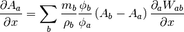
Here  and
and  are the mass of and gas density associated
with the
are the mass of and gas density associated
with the  ’th particle,
  is an arbitrary function of
position (common choices are
is an arbitrary function of
position (common choices are  and
and  ), and
  is the
SPH smoothing kernel at the position of particle . The derivative
inside the sum in the above expression is evaluated at the position of particle
.
is the
SPH smoothing kernel at the position of particle . The derivative
inside the sum in the above expression is evaluated at the position of particle
.
Similarly for the gradient, divergence, and curl:
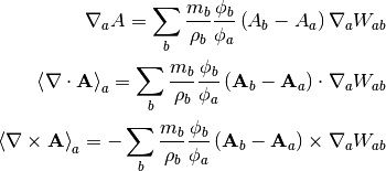
These symmetrized formulae (i.e. they all include a term that looks like
 ) have the advantage that the derivative of a constant field is
zero by construction.
) have the advantage that the derivative of a constant field is
zero by construction.
To actually use these formula, we will need to calculate on a particle-by-particle basis the list of nearest neighbors for each particle and then evaluate these formulae at the locations of each particle. This has not yet been implemented in the version of yt that implements this YTEP, but we expect it to be straightforward using the existing functionality in yt to generate nearest neighbor lists.
Non-local fields that do not depend on an explicit derivative operation will
(e.g. ('gas', 'averaged_density')) will not be implemented for SPH data.
| [PricePaper] | http://adsabs.harvard.edu/abs/2012JCoPh.231..759P |
Data Selection for SPH Fields
Currently data selection for particle fields models all particles, including SPH particles, as infinitesimal points. This means that 2D data objects do not select particles without exact floating point intersection between the data object and the particle.
This YTEP proposes modifying the selection semantics for SPH particles. Instead of modeling SPH particles as infinitesimal points, we will select SPH particles if the smoothing volume intersects with the data container. This means that particles with positions outside of 3D data containers will be selected, since if the smoothing volume overlaps these particles still contribute to estimates of fluid quantities inside of the data object. See Testing for more discussion of the testing strategy used to validate the yt data object and data selection system for SPH particles. To allow for use cases where it is convenient to treat SPH particles as infinitesimal, we will add the ability to dynamically turn on and off this behavior with a configuration option.
We have implemented and added unit tests for all of the following data objects:
- Point
- Slice
- Off-axis Slice
- Region
- Disk
- Ray
In addition, we have implemented the following data object features that depend on hooks in the C selector API:
- Chained selection (e.g.
reg = ds.region(..., data_source=sphere)) - Boolean negation
- Boolean addition
- Boolean AND
- Boolean XOR
ds.intersectionds.union
Visualization of Slices and Projection
Currently slices and projections of SPH data are generated by slicing data that has been SPH smoothed onto the global octree. If there is no more global octree, an alternative strategy for generating pixelized representations of SPH data needs to be implemented. This YTEP proposes replacing the pixelizer operations for slices, off-axis slices, and axis-aligned projections to make use of an SPH-centric pixelization operation. For inspiration, we look to SPLASH, an open-source SPH visualization tool written in Fortran. The algorithms used in SPLASH are detailed in the SPLASH method paper [SPLASHPaper]. We note that we have not consulted the SPLASH source code in support of this implementation.
The key to the pixelization algorithm used in SPLASH is to compute the SPH smoothing operation via the “scatter” approach. Rather than looping over pixels in the image, determining which particles contribute to the SPH smoothing operation at the location of that pixel, and then compute a field value using the SPH smoothing formula, we instead loop over particles, finding the set of pixels whose smoothing volumes overlap with the pixel location and deposit a contribution for that particle to all of the pixels the smoothing volume overlaps. As we loop over all of the particles that contribute to the image, we fill in the image by summing the contributions of each particle. This approach is attractive because it does not require any sort of nearest-neighbor operation and is also trivially parallelizable using e.g. OpenMP threads.
For slices we estimate the contributions of a particle to a single pixel using
the standard SPH smoothing formula. For Projections we make use of a projected
version of the smoothing formula, taking advantage of the spherical symmetry of
the problem. The smoothing operation is implemented in two Cython functions:
pixelize_sph_kernel_slice and pixelize_sph_kernel_projection which are
defined in yt.utilities.lib.pixelization_routines.
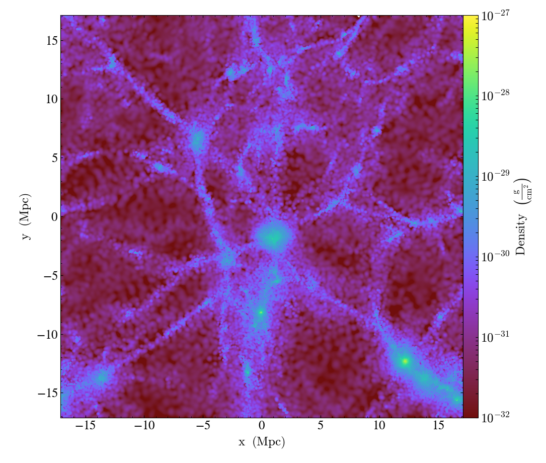
To make the above discussion a bit more concrete, consider the following script:
import yt

ds = yt.load('snapshot_033/snap_033.0.hdf5')

plot = yt.SlicePlot(ds, 2, ('gas', 'density'))

plot.set_zlim(('gas', 'density'), 1e-32, 1e-27)

plot.save()

plot = yt.ProjectionPlot(ds, 2, ('gas', 'density'))

plot.set_zlim(('gas', 'density'), 8e-6, 8e-3)

plot.save()
Running the latest development version of yt at time of writing
(25651334863b) requires 43 seconds to run and produces the following images:
Slice:
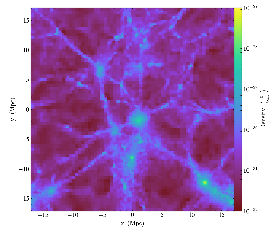
Projection:
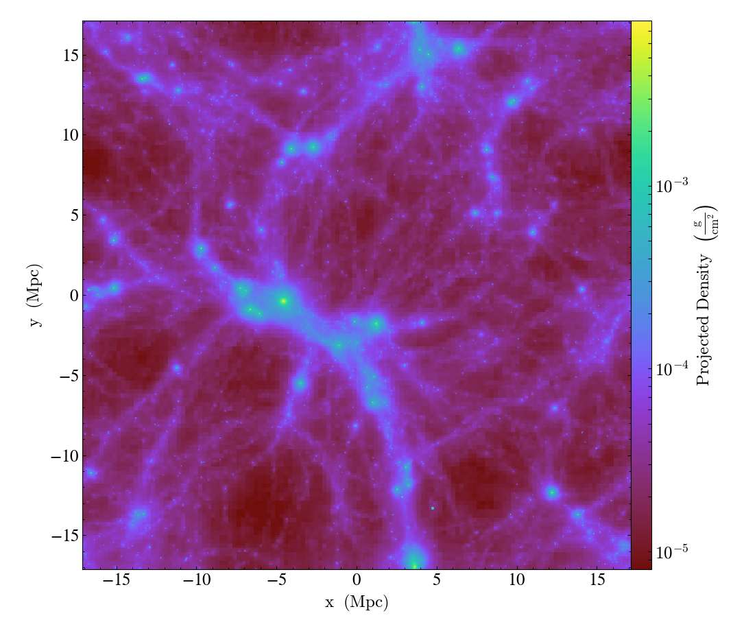
Running the same script on the version of yt that implements this YTEP produces requires 20 seconds and produces the following images:
Slice:
Projection:
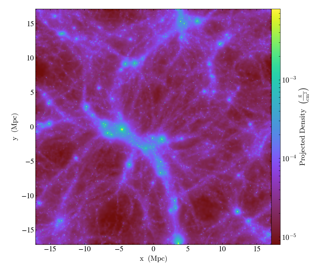
Note also that the performance improvement here becomes more stark for larger datasets as well as for zoom-in simulations which have deeper octrees.
The images produced using the octree are quite “blocky”, since the resolution of
the image in any given location is limited by the octree. This could be
ameliorated somewhat using over_refine_factor but that requires steeper
memory and runtime cost requirements to smooth onto the octree. In general the
images produced by the new pixelizers are truer to the actual structure of the
data. Rather than generating an image from a sampled representation of the real
data, it is our opinion that it makes more sense to instead sample directly from
the particle data.
| [SPLASHPaper] | http://adsabs.harvard.edu/doi/10.1071/AS07022 |
Deposition operations
Regular Grids
While we do want to make it easier to access particle-centric data, we need to
make sure it’s still possible to locally deposit and SPH smooth data onto
grids. Not only is that a useful operation for users of SPH codes, but it’s also
functionality that yt currently provides, so we need to ensure that currently
supported operations on covering_grid and arbitrary_grid data objects
continue to work and produce sensible results. We will add tests to verify that
this is the case.
Octrees
We should not abandon the ability to smooth SPH data and deposit particle data onto a volume-filling octree. Simply because users are currently using these data for their own analyses, we need to provide a migration path so that users can reproduce prior work made with yt using the global octree.
We propose adding a new data object to yt that represents an octree with a given
bounding box (which need not overlap with the domain bounding box) and maximum
refinement level. One can think of this as something of an adaptive
arbitrary_grid data object. Initially we will only allow refinement in terms
of particle quantities (e.g. particle mass or particle count per octree leaf
node), but it should be possible to add support for data defined on octree or
patch AMR meshes eventually.
We still need to decide on an appropriate API for this. Ideally we would be able to reuse some of the existing code for the global octree.
Testing
The testing strategy for this work follows two basic approaches so far. First,
we make sure that all derived fields that are associated with a number of
real-world SPH datasets from http://yt-project.org/data can be calculated
without generating any errors. This ensures both that the derived field system
is functioning but also that the I/O routines in the various SPH frontends are
functioning correctly. These tests are present in
yt.fields.tests.test_sph_fields.
In addition, we have added support in the stream frontend for loading SPH
data. This allows us to create fake in-memory SPH datasets that we can construct
in a way that make them easier to reason about for testing than a real-world SPH
dataset. The primary route for generating these dataset is a new function in the
yt.testing namespace, fake_sph_orientation_ds. This function has the
following very straightforward definition:
def fake_sph_orientation_ds():
    """Returns an in-memory SPH dataset useful for testing

    This dataset should have one particle at the origin, one more particle
    along the x axis, two along y, and three along z. All particles will
    have non-overlapping smoothing regions with a radius of 0.25, masses of 1,
    and densities of 1, and zero velocity.
    """
    from yt import load_particles

    npart = 7

    # one particle at the origin, one particle along x-axis, two along y,
    # three along z
    data = {
        'particle_position_x': (
            np.array([0.0, 1.0, 0.0, 0.0, 0.0, 0.0, 0.0]), 'cm'),
        'particle_position_y': (
            np.array([0.0, 0.0, 1.0, 2.0, 0.0, 0.0, 0.0]), 'cm'),
        'particle_position_z': (
            np.array([0.0, 0.0, 0.0, 0.0, 1.0, 2.0, 3.0]), 'cm'),
        'particle_mass': (np.ones(npart), 'g'),
        'particle_velocity_x': (np.zeros(npart), 'cm/s'),
        'particle_velocity_y': (np.zeros(npart), 'cm/s'),
        'particle_velocity_z': (np.zeros(npart), 'cm/s'),
        'smoothing_length': (0.25*np.ones(npart), 'cm'),
        'density': (np.ones(npart), 'g/cm**3'),
    }

    bbox = np.array([[-4, 4], [-4, 4], [-4, 4]])

    return load_particles(data=data, length_unit=1.0, bbox=bbox)
This example also demonstrates how load_particles can be used by users in
this work to load SPH data written in data formats that aren’t yet supported by
a frontend. This testing dataset has one particle at the origin, another
particle along the x axis, two more along the y axis, and three along z. All
particles have the same smoothing length, such that the smoothing volumes of any
of the particles in the dataset do not overlap. This means that we can construct
various data objects and reason about which particles we should be selecting
given the geometry of the particles in the dataset and the boundaries of the
data object. In addition, we take care to make sure that the boundaries of the
data objects do not necessarily directly overlap with the position of a particle
near the boundary. This ensures that particles are selected when their smoothing
volume overlaps with a data object, not necessarily based on the particle
positions. These tests are present in
yt.data_objects.tests.test_sph_data_objects. Currently all of the data
objects supported by yt are explicitly tested here. As an example, here is the
test that verifies the slice data object is working correctly:
# The number of particles along each slice axis at that coordinate
SLICE_ANSWERS = {
    ('x', 0): 6,
    ('x', 0.5): 0,
    ('x', 1): 1,
    ('y', 0): 5,
    ('y', 1): 1,
    ('y', 2): 1,
    ('z', 0): 4,
    ('z', 1): 1,
    ('z', 2): 1,
    ('z', 3): 1,
}

def test_slice():
    ds = fake_sph_orientation_ds()
    for (ax, coord), answer in SLICE_ANSWERS.items():
        # test that we can still select particles even if we offset the slice
        # within each particle's smoothing volume
        for i in range(-1, 2):
            sl = ds.slice(ax, coord + i*0.1)
            assert_equal(sl['gas', 'density'].shape[0], answer)
Open Questions
There are a number of design decisions that still need to be made if this YTEP is going to be fully implemented and accepted. Comments and suggestions on these points are very welcome.
The Projection Data Object
Currently the projection data object is completely broken for particle data for all frontends:
In [1]: import yt

In [2]: ds = yt.load('IsolatedGalaxy/galaxy0030/galaxy0030')
yt : [INFO     ] 2017-03-01 09:54:22,491 Parameters: current_time              = 0.0060000200028298
yt : [INFO     ] 2017-03-01 09:54:22,491 Parameters: domain_dimensions         = [32 32 32]
yt : [INFO     ] 2017-03-01 09:54:22,492 Parameters: domain_left_edge          = [ 0.  0.  0.]
yt : [INFO     ] 2017-03-01 09:54:22,492 Parameters: domain_right_edge         = [ 1.  1.  1.]
yt : [INFO     ] 2017-03-01 09:54:22,492 Parameters: cosmological_simulation   = 0.0

In [3]: proj = ds.proj(('gas', 'density'), 0)
Parsing Hierarchy : 100%|████████████████████| 173/173 [00:00<00:00, 3535.74it/s]
yt : [INFO     ] 2017-03-01 09:54:27,650 Gathering a field list (this may take a moment.)
yt : [INFO     ] 2017-03-01 09:54:29,653 Projection completed

In [4]: proj['all', 'particle_mass']
---------------------------------------------------------------------------
ValueError                                Traceback (most recent call last)
<ipython-input-4-1a26d598985b> in <module>()
----> 1 proj['all', 'particle_mass']

/Users/goldbaum/Documents/yt-hg/yt/data_objects/data_containers.py in __getitem__(self, key)
    281                 return self.field_data[f]
    282             else:
--> 283                 self.get_data(f)
    284         # fi.units is the unit expression string. We depend on the registry
    285         # hanging off the dataset to define this unit object.

/Users/goldbaum/Documents/yt-hg/yt/data_objects/construction_data_containers.py in get_data(self, fields)
    339                     self._initialize_projected_units(fields, chunk)
    340                     _units_initialized = True
--> 341                 self._handle_chunk(chunk, fields, tree)
    342         # Note that this will briefly double RAM usage
    343         if self.method == "mip":

/Users/goldbaum/Documents/yt-hg/yt/data_objects/construction_data_containers.py in _handle_chunk(self, chunk, fields, tree)
    440         v = np.empty((chunk.ires.size, len(fields)), dtype="float64")
    441         for i, field in enumerate(fields):
--> 442             d = chunk[field] * dl
    443             v[:,i] = d
    444         if self.weight_field is not None:

/Users/goldbaum/Documents/yt-hg/yt/units/yt_array.py in __mul__(self, right_object)
    955         """
    956         ro = sanitize_units_mul(self, right_object)
--> 957         return super(YTArray, self).__mul__(ro)
    958
    959     def __rmul__(self, left_object):

ValueError: operands could not be broadcast together with shapes (3976,) (37432,)
By making SPH data return most data as particle fields we are making this
problem much more visible. We should decide what a sensible return value for the
projection operation on a particle field should be. Note that in practice we do
not need to solve this issue to create a ProjectionPlot since we can
short-circuit the data selection operation when we create the pixelized
projection.
Some ideas:
- Write a new
ParticleQuadTreeclass that adaptively deposits particle data onto a quadtree mesh. - Since most people really want a pixelized representation of the particle data
(e.g. via a
FixedResolutionBufferwe could simply make it so the projection data object returns a regular resolution image.
Cut Regions
We have not yet implemented the Cut Region data object since it’s not clear how it should work for particle data. Similar to the projection data object, the cut region data object does not currently work when it is defined in terms of a threshold on a particle field. It may be possible to define an internal particle filter to implement cuts on Lagrangian data.
Volume Rendering
Currently we don’t support volume rendering particle data. In principle writing at least a basic volume renderer specifically for particle data is a straightforward project. Making it scale well to arbitrarily large datasets would be a bigger undertaking, but we think we should attempt to write a volume rendering engine that accepts particle data. Optimally this will plug in to the existing volume rendering infrastructure at the same level as the AMRKDTree. Attempting this will also make it easier to add support for volume rendering octree AMR data with an octree volume rendering engine.
The API and design for this component have not yet been settled.
Community engagement
We are early enough in the process of implementing this YTEP that the major design points have not yet calcified. To encourage wide adoption of these changes with a minimum amount of breakage for existing users, we will to reach out to existing users of yt who regularly work with SPH data to ensure that their existing code continue to work as much as possible. If there are widespread breakages, this will inform where we should focus on building backward compatibility shims and helpers.
Before this work can be merged into the main development branch we will need to update the documentation for particle data. This should include coverage of the following topics:
- Loading in-memory SPH data using
load_particles - A high-level description of the Morton bitmap index system and how to tune it for performance by adjusting the maximum coarse and refined Morton index level.
- A high-level description of the data selection semantics for particle and SPH data.
- A transition guide explaining all of the changes and how to port scripts, particularly those making direct use of the global octree via a deposition operation.
Finally, we will attempt to publicize this document as much as possible to attract feedback from current and prospective users at an early stage.
yt 4.0?
Since these are substantial backward incompatible changes, we think the next version of yt released after this work is merged should be yt 4.0. This opens the possibility of adding other backward incompatible changes as well as removing deprecated features. We should be sure to signal to our users that there will only be major changes for those who work with SPH data - support for AMR and unstructured mesh data should remain the same.